(and other things that go bump in the night)
A variety of statistical procedures exist. The appropriate statistical procedure depends on the research question(s) we are asking and the type of data we collected. While EPSY 5601 is not intended to be a statistics class, some familiarity with different statistical procedures is warranted.
Parametric Data Analysis
Investigating Differences
One Independent Variable (With Two Levels) and One Dependent Variable
When we wish to know whether the means of two groups (one independent variable (e.g., gender) with two levels (e.g., males and females) differ, a t test is appropriate. In order to calculate a t test, we need to know the mean, standard deviation, and number of subjects in each of the two groups. An example of a t test research question is “Is there a significant difference between the reading scores of boys and girls in sixth grade?” A sample answer might be, “Boys (M=5.67, SD=.45) and girls (M=5.76, SD=.50) score similarly in reading, t(23)=.54, p>.05.” [Note: The (23) is the degrees of freedom for a t test. It is the number of subjects minus the number of groups (always 2 groups with a t-test). In this example, there were 25 subjects and 2 groups so the degrees of freedom is 25-2=23.] Remember, a t test can only compare the means of two groups (independent variable, e.g., gender) on a single dependent variable (e.g., reading score). You may wish to review the instructor notes for t tests.
One Independent Variable (With More Than Two Levels) and One Dependent Variable
If the independent variable (e.g., political party affiliation) has more than two levels (e.g., Democrats, Republicans, and Independents) to compare and we wish to know if they differ on a dependent variable (e.g., attitude about a tax cut), we need to do an ANOVA (ANalysis Of VAriance). In other words, if we have one independent variable (with three or more groups/levels) and one dependent variable, we do a one-way ANOVA. A sample research question is, “Do Democrats, Republicans, and Independents differ on their option about a tax cut?” A sample answer is, “Democrats (M=3.56, SD=.56) are less likely to favor a tax cut than Republicans (M=5.67, SD=.60) or Independents (M=5.34, SD=.45), F(2,120)=5.67, p<.05.” [Note: The (2,120) are the degrees of freedom for an ANOVA. The first number is the number of groups minus 1. Because we had three political parties it is 2, 3-1=2. The second number is the total number of subjects minus the number of groups. Because we had 123 subject and 3 groups, it is 120 (123-3)]. The one-way ANOVA has one independent variable (political party) with more than two groups/levels (Democrat, Republican, and Independent) and one dependent variable (attitude about a tax cut).
More Than One Independent Variable (With Two or More Levels Each) and One Dependent Variable
ANOVAs can have more than one independent variable. A two-way ANOVA has two independent variable (e.g. political party and gender), a three-way ANOVA has three independent variables (e.g., political party, gender, and education status), etc. These ANOVA still only have one dependent variable (e.g., attitude about a tax cut). A two-way ANOVA has three research questions: One for each of the two independent variables and one for the interaction of the two independent variables.
Sample Research Questions for a Two-Way ANOVA:
Do Democrats, Republicans, and Independents differ on their opinion about a tax cut?
Do males and females differ on their opinion about a tax cut?
Is there an interaction between gender and political party affiliation regarding opinions about a tax cut?
A two-way ANOVA has three null hypotheses, three alternative hypotheses and three answers to the research question. The answers to the research questions are similar to the answer provided for the one-way ANOVA, only there are three of them.
One or More Independent Variables (With Two or More Levels Each) and More Than One Dependent Variable
Sometimes we have several independent variables and several dependent variables. In this case we do a MANOVA (Multiple ANalysis Of VAriance). Suffices to say, multivariate statistics (of which MANOVA is a member) can be rather complicated.
Investigating Relationships
Simple Correlation
Sometimes we wish to know if there is a relationship between two variables. A simple correlation measures the relationship between two variables. The variables have equal status and are not considered independent variables or dependent variables. In our class we used Pearson‘s r which measures a linear relationship between two continuous variables. While other types of relationships with other types of variables exist, we will not cover them in this class. A sample research question for a simple correlation is, “What is the relationship between height and arm span?” A sample answer is, “There is a relationship between height and arm span, r(34)=.87, p<.05.” You may wish to review the instructor notes for correlations. A canonical correlation measures the relationship between sets of multiple variables (this is multivariate statistic and is beyond the scope of this discussion).
Regression
An extension of the simple correlation is regression. In regression, one or more variables (predictors) are used to predict an outcome (criterion). One may wish to predict a college student’s GPA by using his or her high school GPA, SAT scores, and college major. Data for several hundred students would be fed into a regression statistics program and the statistics program would determine how well the predictor variables (high school GPA, SAT scores, and college major) were related to the criterion variable (college GPA). Based on the information, the program would create a mathematical formula for predicting the criterion variable (college GPA) using those predictor variables (high school GPA, SAT scores, and/or college major) that are significant. Not all of the variables entered may be significant predictors. A sample research question might be, “What is the individual and combined power of high school GPA, SAT scores, and college major in predicting graduating college GPA?” The output of a regression analysis contains a variety of information. R2tells how much of the variation in the criterion (e.g., final college GPA) can be accounted for by the predictors (e.g., high school GPA, SAT scores, and college major (dummy coded 0 for Education Major and 1 for Non-Education Major). A research report might note that “High school GPA, SAT scores, and college major are significant predictors of final college GPA, R2=.56.” In this example, 56% of an individual’s college GPA can be predicted with his or her high school GPA, SAT scores, and college major). The regression equation for such a study might look like the following: Y’= .15 + (HS GPA * .75) + (SAT * .001) + (Major * -.75). By inserting an individual’s high school GPA, SAT score, and college major (0 for Education Major and 1 for Non-Education Major) into the formula, we could predict what someone’s final college GPA will be (well…at least 56% of it). For example, someone with a high school GPA of 4.0, SAT score of 800, and an education major (0), would have a predicted GPA of 3.95 (.15 + (4.0 * .75) + (800 * .001) + (0 * -.75)). Universities often use regression when selecting students for enrollment.
I have created a sample SPSS regression printout with interpretation if you wish to explore this topic further. You will not be responsible for reading or interpreting the SPSS printout.
Non Parametric Data Analysis
Chi-Square
We might count the incidents of something and compare what our actual data showed with what we would expect. Suppose we surveyed 27 people regarding whether they preferred red, blue, or yellow as a color. If there were no preference, we would expect that 9 would select red, 9 would select blue, and 9 would select yellow. We use a chi-square to compare what we observe (actual) with what we expect. If our sample indicated that 2 liked red, 20 liked blue, and 5 liked yellow, we might be rather confident that more people prefer blue. If our sample indicated that 8 liked read, 10 liked blue, and 9 liked yellow, we might not be very confident that blue is generally favored. Chi-square helps us make decisions about whether the observed outcome differs significantly from the expected outcome. A sample research question is, “Is there a preference for the red, blue, and yellow color?” A sample answer is “There was not equal preference for the colors red, blue, or yellow. More people preferred blue than red or yellow, X2 (2) = 12.54, p < .05″. Just as t-tests tell us how confident we can be about saying that there are differences between the means of two groups, the chi-square tells us how confident we can be about saying that our observed results differ from expected results.
In Summary
Each of the stats produces a test statistic (e.g., t, F, r, R2, X2) that is used with degrees of freedom (based on the number of subjects and/or number of groups) that are used to determine the level of statistical significance (value of p). Ultimately, we are interested in whether p is less than or greater than .05 (or some other value predetermined by the researcher). It all boils down the the value of p. If p<.05 we say there are differences for t-tests, ANOVAs, and Chi-squares or there are relationships for correlations and regressions.
Model Building
Thanks to improvements in computing power, data analysis has moved beyond simply comparing one or two variables into creating models with sets of variables. Structural Equation Modeling and Hierarchical Linear Modeling are two examples of these techniques. Structural Equation Modeling (SEM) analyzes paths between variables and tests the direct and indirect relationships between variables as well as the fit of the entire model of paths or relationships. For example, a researcher could measure the relationship between IQ and school achievment, while also including other variables such as motivation, family education level, and previous achievement.
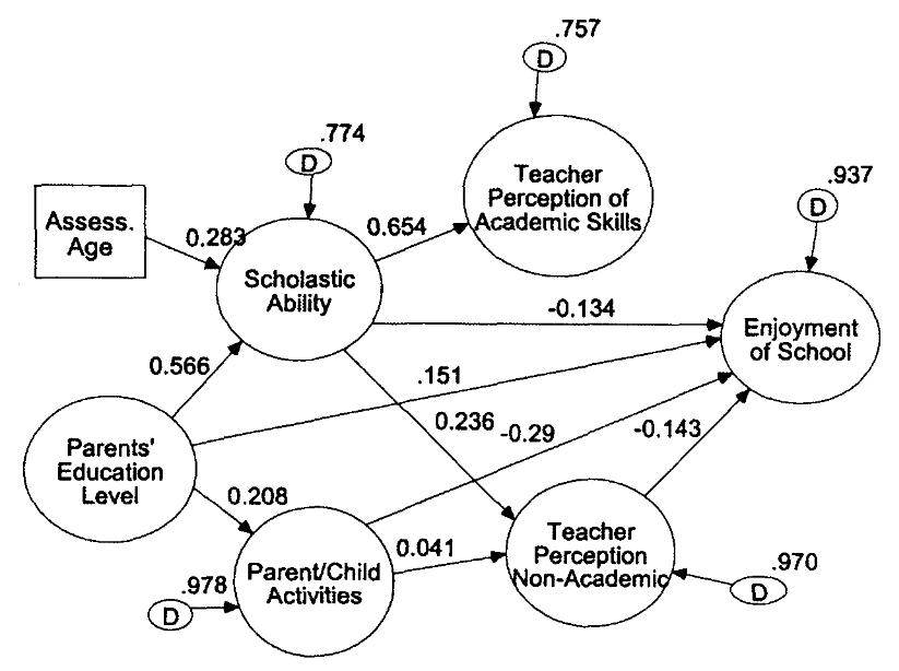
The example below shows the relationships between various factors and enjoyment of school. When a line (path) connects two variables, there is a relationship between the variables. If two variable are not related, they are not connected by a line (path). The strengths of the relationships are indicated on the lines (path). In this model we can see that there is a positive relationship between Parents’ Education Level and students’ Scholastic Ability. We can see that there is not a relationship between Teacher Perception of Academic Skills and students’ Enjoyment of School. We can see there is a negative relationship between students’ Scholastic Ability and their Enjoyment of School. See D. Betsy McCoach’s article for more information on Structural Equation Modeling (SEM) in Gifted Education.
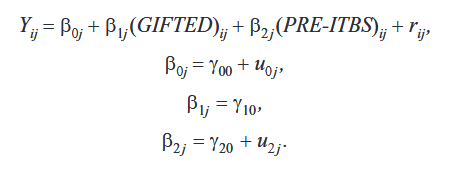
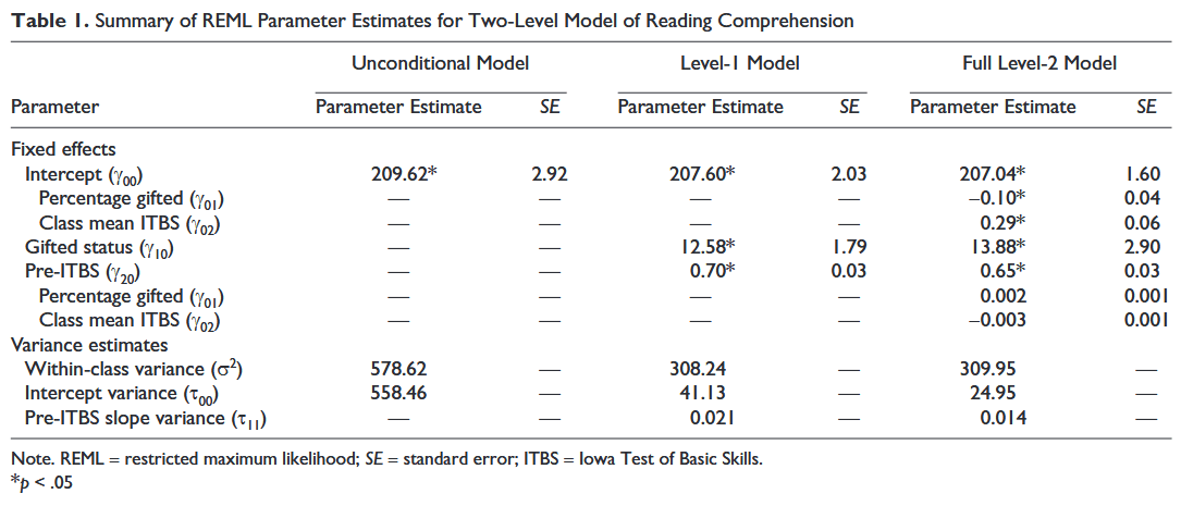
Often the educational data we collect violates the important assumption of independence that is required for the simpler statistical procedures. Students are often grouped (nested) in classrooms. Those classrooms are grouped (nested) in schools. The schools are grouped (nested) in districts. This nesting violates the assumption of independence because individuals within a group are often similar. Hierarchical Linear Modeling (HLM) was designed to work with nested data. HLM allows researchers to measure the effect of the classroom, as well as the effect of attending a particular school, as well as measuring the effect of being a student in a given district on some selected variable, such as mathematics achievement. For more information on HLM, see D. Betsy McCoach’s article on Introduction to Hierarchical Linear Modeling.
Del Siegle
del.siegle@uconn.edu


