The PowerPoint presentation contains important information for this unit on correlations. Contact the instructor, del.siegle@uconn.edu…if you have trouble viewing it.
Some content on this website may require the use of a plug-in, such as Microsoft PowerPoint.
When are correlation methods used?
- They are used to determine the extent to which two or more variables are related among a single group of people (although sometimes each pair of score does not come from one person…the correlation between father’s and son’s height would not).
- There is no attempt to manipulate the variables (random variables)
How is correlational research different from experimental research?
In correlational research we do not (or at least try not to) influence any variables but only measure them and look for relations (correlations) between some set of variables, such as blood pressure and cholesterol level. In experimental research, we manipulate some variables and then measure the effects of this manipulation on other variables; for example, a researcher might artificially increase blood pressure and then record cholesterol level. Data analysis in experimental research also comes down to calculating “correlations” between variables, specifically, those manipulated and those affected by the manipulation. However, experimental data may potentially provide qualitatively better information: Only experimental data can conclusively demonstrate causal relations between variables. For example, if we found that whenever we change variable A then variable B changes, then we can conclude that “A influences B.” Data from correlational research can only be “interpreted” in causal terms based on some theories that we have, but correlational data cannot conclusively prove causality.Source: http://www.statsoft.com/textbook/stathome.html
Although a relationship between two variables does not prove that one caused the other, if there is no relationship between two variables then one cannot have caused the other.
Correlation research asks the question: What relationship exists?
- A correlation has direction and can be either positive or negative (note exceptions listed later). With a positive correlation, individuals who score above (or below) the average (mean) on one measure tend to score similarly above (or below) the average on the other measure. The scatterplot of a positive correlation rises (from left to right). With negative relationships, an individual who scores above average on one measure tends to score below average on the other (or vise verse). The scatterplot of a negative correlation falls (from left to right).
- A correlation can differ in the degree or strength of the relationship (with the Pearson product-moment correlation coefficient that relationship is linear). Zero indicates no relationship between the two measures and r = 1.00 or r = -1.00 indicates a perfect relationship. The strength can be anywhere between 0 and + 1.00. Note: The symbol r is used to represent the Pearson product-moment correlation coefficient for a sample. The Greek letter rho (r) is used for a population. The stronger the correlation–the closer the value of r (correlation coefficient) comes to + 1.00–the more the scatterplot will plot along a line.
When there is no relationship between the measures (variables), we say they are unrelated, uncorrelated, orthogonal, or independent.
Some Math for Bivariate Product Moment Correlation (not required for EPSY 5601):
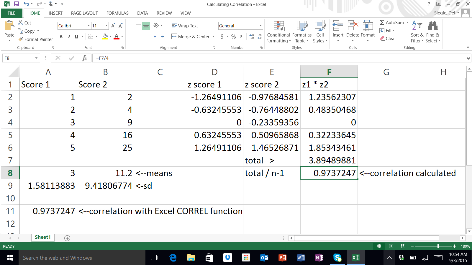
Multiple the z scores of each pair and add all of those products. Divide that by one less than the number of pairs of scores. (pretty easy)
—or—
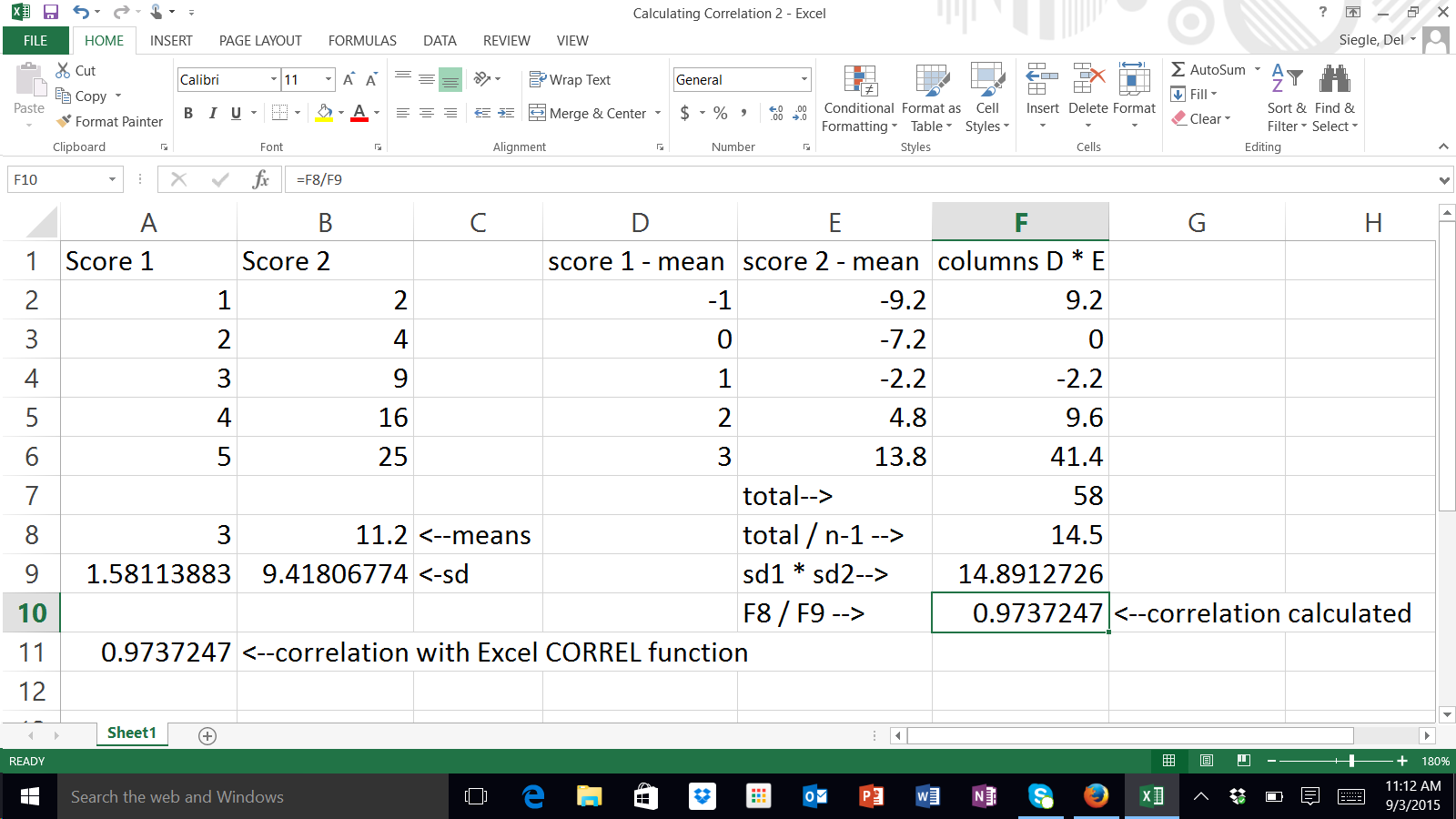
Each pair has two scores…one from each of two variables. For each pair, subtract the mean for each variable from the pair’s score on that variable and multiply the results times each other–> (Score1 – Mean1) * (Score2 – Mean2). Total those results for all of the pairs –> SUM((Score1 – Mean1) * (Score2 – Mean2)). Divide that by the number of pairs minus 1–>SUM((Score1 – Mean1) * (Score2 – Mean2)) / (n – 1). Multiple the standard deviation for each of the two variables times each other and divide your previous answer by that –> (SUM((Score1 – Mean1) * (Score2 – Mean2)) / (n – 1)) / (SD1 * SD2).
Rather than calculating the correlation coefficient with either of the formulas shown above, you can simply follow these linked directions for using the function built into Microsoft’s Excel.
Some correlation questions elementary students can investigate are
What is the relationship between…
- school attendance and grades in school?
- hours spend each week doing homework and school grades?
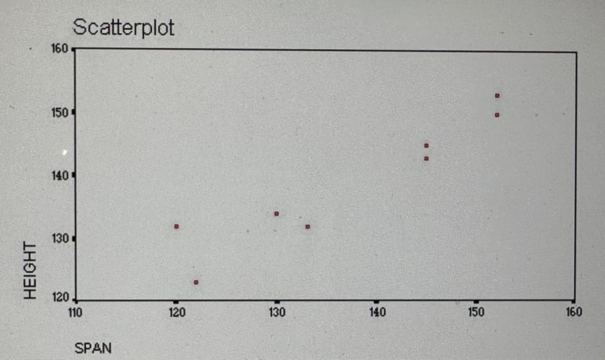
- length of arm span and height?
- number of children in a family and the number of bedrooms in the house?
Correlations only describe the relationship, they do not prove cause and effect. Correlation is a necessary, but not a sufficient condition for determining causality.
There are Three Requirements to Infer a Causal Relationship
- A statistically significant relationship between the variables
- The causal variable occurred prior to the other variable
- There are no other factors that could account for the cause
(Correlation studies do not meet the last requirement and may not meet the second requirement. However, not having a relationship does mean that one variable did not cause the other.)
There is a strong relationship between the number of ice cream cones sold and the number of people who drown each month. Just because there is a relationship (strong correlation) does not mean that one caused the other.
If there is a relationship between A (ice cream cone sales) and B (drowning) it could be because
- A->B (Eating ice cream causes drowning)
- A<-B (Drowning cause people to eat ice cream– perhaps the mourners are so upset that they buy ice cream cones to cheer themselves)
- A<-C->B (Something else is related to both ice cream sales and the number of drowning– warm weather would be a good guess)
The points is…just because there is a correlation, you CANNOT say that the one variable causes the other. On the other hand, if there is NO correlations, you can say that one DID NOT cause the other (assuming the measures are valid and reliable).
Format for correlations research questions and hypotheses:
Question: Is there a (statistically significant) relationship between height and arm span?
HO: There is no (statistically significant) relationship between height and arm span (H0: r=0).
HA: There is a (statistically significant) relationship between height and arm span (HA: r<>0).
Coefficient of Determination (Shared Variation)
One way researchers often express the strength of the relationship between two variables is by squaring their correlation coefficient. This squared correlation coefficient is called a COEFFICIENT OF DETERMINATION. The coefficient of determination is useful because it gives the proportion of the variance of one variable that is predictable from the other variable.
Factors which could limit a product-moment correlation coefficient (PowerPoint demonstrating these factors)
- Homogenous group (the subjects are very similar on the variables)
- Unreliable measurement instrument (your measurements can’t be trusted and bounce all over the place)
- Nonlinear relationship (Pearson’s r is based on linear relationships…other formulas can be used in this case)
- Ceiling or Floor with measurement (lots of scores clumped at the top or bottom…therefore no spread which creates a problem similar to the homogeneous group)
Assumptions one must meet in order to use the Pearson product-moment correlation
- The measures are approximately normally distributed
- The variance of the two measures is similar (homoscedasticity) — check with scatterplot
- The relationship is linear — check with scatterplot
- The sample represents the population
- The variables are measured on a interval or ratio scale
There are different types of relationships: Linear – Nonlinear or Curvilinear – Non-monotonic (concave or cyclical). Different procedures are used to measure different types of relationships using different types of scales. The issue of measurement scales is very important for this class. Be sure that you understand them.
Predictor and Criterion Variables (NOT NEEDED FOR EPSY 5601)
- Multiple Correlation- lots of predictors and one criterion (R)
- Partial Correlation- correlation of two variables after their correlation with other variables is removed
- Serial or Autocorrelation- correlation of a set of number with itself (only staggered one)
- Canonical Correlation- lots of predictors and lots of criterion Rc
When using a critical value table for Pearson’s product-moment correlation, the value found through the intersection of degree of freedom (n – 2) and the alpha level you are testing (p = .05) is the minimum r value needed in order for the relationship to be above chance alone.
The statistics package SPSS as well as Microsoft’s Excel can be used to calculate the correlation.
We will use Microsoft’s Excel.
Reading a Correlations Table in a Journal Article
Most research studies report the correlations among a set of variables. The results are presented in a table such as the one shown below.
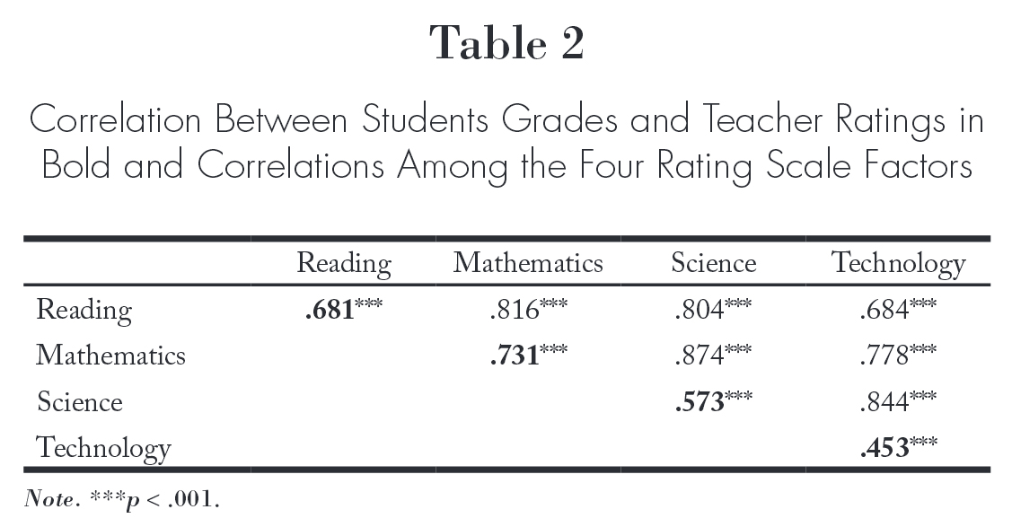
The intersection of a row and column shows the correlation between the variable listed for the row and the variable listed for the column. For example, the intersection of the row mathematics and the column science shows that the correlation between mathematics and science was .874. The footnote states that the three *** after .874 indicate the relationship was statistically significant at p<.001.
Most tables do not report the perfect correlation along the diagonal that occurs when a variable is correlated with itself. In the example above, the diagonal was used to report the correlation of the four factors with a different variable. Because the correlation between reading and mathematics can be determined in the top section of the table, the correlations between those two variables is not repeated in the bottom half of the table. This is true for all of the relationships reported in the table. .
Del Siegle, Ph.D.
Neag School of Education – University of Connecticut
del.siegle@uconn.edu
www.delsiegle.com
Last updated 10/11/2015