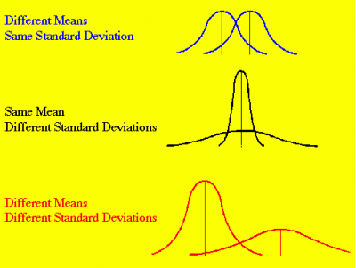
I created a PowerPoint on the normal distribution to teach some of the concepts covered in this unit.
There are three different MEASURES of CENTRAL TENDENCY (check out this link)
(Ways to be average)
- Mean=arithmetic average of a set of scores
(add all of the scores and divide by the number of scores you used)
(i.e., 3, 11, 3, 4, 7, 8 –> 3 + 11 + 3 + 4 + 7 + 8 = 36 –> 36 divided by 6 (number of scores) = 6) - Mode= score that appears most often
(i.e., 3, 11, 3, 4, 7, 8 –> there are more 3s than any other value so 3 is the mode) - Median= middle score when the scores are put in order of value
(i.e., 3, 11, 3, 4, 7, 8 –> 3, 3, 4, 7, 8, 11 (scores in order) –> the middle is between 4 and 7 so the median is 5.5 (half way between 4 and 7)
MEASURES of VARIATION (Spread)
- Range=difference between the high and low score (i.e., 3, 11, 3, 4, 7, 8 –> 3, 3, 4, 7, 8, 11 (scores in order) –> 11 (high) minus 3 (low) = 8
- Variance=average of the squared distance each score is from the mean
(i.e., 3, 11, 3, 4, 7, 8)
(The mean is 6 and we subtract 6 from each score and then square that answer) –>
3 – 6 = -3 –> -3 X -3 = 9
11 – 6 = 5 –> 5 X 5 = 25
3 – 6 = -3 –> -3 X -3 = 9
4 – 6 = -2 –> -2 X -2 = 4
7 – 6 = 1 –> 1 X 1 = 1
8 – 6 = 2 –> 2 X 2 = 4
(Now we add all of the squared scores) –> 9 + 25 + 9 + 4 + 1 + 4 = 52
(Next we divide this total (total of the squared distance each score was from the mean) by the number of scores) –> 52 divided by 6 (number of scores) = 8.67NOTE: We divide by number of scores if the data is from the entire population…we divide by the number of scores minus 1 (6-1=5) if the data is from a sample. If our data were from a sample the variance would be 52 divided by 5 (52 divided by 5 = 10.4) - Standard Deviation =square root of the variance
(i.e., 3, 11, 3, 4, 7, 8 –> has a variance of 8.67 for a population so the standard deviation the square root of 8.67 or 2.94 (use a calculator to find it))
(i.e., 3, 11, 3, 4, 7, 8 –> has a variance of 10.4 for a sample so the standard deviation is the square root of 10.4 or 3.22 (use a calculator to find it))
YOU CAN EASILY CALCULATE THE MEAN AND STANDARD DEVIATION WITH EXCEL.
Properties of the Normal Distribution
- Unimodal (one mode)
- Symmetrical (left and right halves are mirror images)– just as many people above the mean as below the mean
- Bell shaped (maximum height (mode) at the mean)
- Mean, Mode, and Median are all located in the center
- Asymptotic (the further the curve goes from the mean, the closer it gets to the X axis; but the curve never touches the X axis)
AREA UNDER the NORMAL CURVE
- 68% of our subjects are plus or minus one standard deviation
- 95.4% of our subjects are plus or minus two standard deviations
- 99.7% of our subjects are plus or minus three standard deviations
Assuming that we have a normal distribution, it is easy to calculate what percentage of students who are between 1.5 standard deviations above the mean and 2.5 standard deviations above the mean. To do this, use the Area Under the Normal Curve Calculator at https://davidmlane.com/hyperstat/z_table.html.
Please check this link on STANDARDIZED SCORES to learn why they are meaningful
A z score indicates the number of standard deviations a corresponding raw score is above or below the mean
z score –> subtract the mean from the raw score and divide that answer by the standard deviation
(i.e., raw score=5, mean=8, standard deviation=2 –> 5 – 8 = -3 –> -3 divided by 2 = -1.5)
T score (transformed score — a.k.a. Z score) –> multiple the z score by 10 and add 50
(i.e., z score=-1.5 –> -1.5 X 10 = -15 –> -15 + 50 = 35)
Scores don’t always form a normal distribution

The skew is the tail. If the tail (skew) is on the left (negative side), we have a negatively skewed distribution. That means that more of the subjects scored on the high end (because most of the people are not in the tail where the low scores are)..
If the skew (tail) is on the right (positive side), we have a positive skew. That means more people scored low (because most of the people are not in the tail where the high scores are).
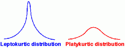
Sometimes most of the scores are in the middle, we then have a leptokurtic distribution.
Sometimes the scores have a large spread without a lot of people in the middle, we then have a platykurtic distribution.
If a set of scores does not form a normal distribution (skewed), then the characteristics of the normal curve do not apply. For example, 68% of the scores would not fall within one standard deviation of the mean if the distribution were negatively skewed.
Del Siegle, Ph.D.
Neag School of Education – University of Connecticut
del.siegle@uconn.edu

![Normal Distribution Curve [-3 SD (between 0.13% to 2.14%); -2 SD (between 2.14% to 13.59%); -1 SD (between 13.59% to 34.13%); 0 (between 34.13% to 34.13%); +1 SD (between 34.13% to 13.59%); +2 SD (between 13.59% to 2.14%); +3 SD (between 2.14% to 0.13%)]](https://researchbasics-education.media.uconn.edu/wp-content/uploads/sites/1215/2015/05/normal-400x185.gif)
![Area Under the normal Curve: Normal Distribution Curve from HyperStat Online Home Page: [Checked selection] Area from a value (Use to compute p from Z) [Unchecked selection] Value from an area (Use to compute Z for confidence intervals) Specify Parameters: Mean: 0, SD: 1, [Unchecked selection] Above: 1.96, [Unchecked selection] Below: 1.96, [Checked selection] Between: 1.5 and 2.5, [Unchecked selection] Outside: -1.96 and 1.96, Results: Area (probability): 0.0606, Recalculate Button. Enter 1.5 {An arrow pointing to the 1.5 in the Between selection} and 2.5 {An arrow pointing to the 2.5 in the Between selection} and click on the Between (Bold) radio {An arrow pointing to the Between selection} button. Approximately 6% {An arrow pointing to the Area (Probability) section} of students would be between 1.5 to 2.5.](https://researchbasics-education.media.uconn.edu/wp-content/uploads/sites/1215/2015/05/AreaUnderCurve.jpg)
